Extrapolation in Conditional Generation of Molecules
Published:
Out-of-Distribution (OOD) generalization in conditional generation of molecules - a case study.
Motivation for Out-of-Distribution (OOD) Generalization for Materials
Developing new materials and molecules is a cornerstone of technological innovation. From semiconductors to bio-degradable polymers, the ability to tailor materials with specific properties underpins advances across industries. There is particular interest in property values that are outside the known property value distribution as these will most likely lead to discovering new materials that will, in turn, unlock new capabilities and technologies.
For instance, in solar energy, discovering solid-state materials with enhanced energy conversion efficiency could lead to substantial improvements in the performance of solar panels, contributing to more sustainable energy solutions. In healthcare, discovering drug molecules with exceptional binding affinities or novel biological activities could open new avenues for treating diseases that currently lack effective therapies, thus advancing the medical field. In environmental sustainability, materials with exceptional carbon dioxide adsorption capacities could greatly improve carbon capture technologies, helping to reduce greenhouse gas emissions and combat climate change.
The discovery of such materials, those with properties beyond the range of materials already known and characterized, holds the promise of addressing pressing challenges in modern technology.
OOD What?
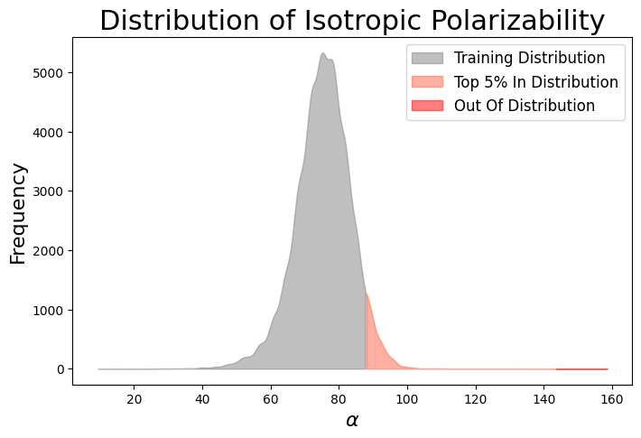
When considering OOD generalization for materials, one can assess the uniqueness of generated materials in relation to the chemical or structural space of the training data, or evaluate the uniqueness of the property values of these materials. In our context, OOD materials are defined as those with property values that fall outside the distribution of the known data (i.e., training data). These materials may also correspond to novel chemical or structural spaces, though this is not always the case.
Case Study: EDM model
EDM is an E(3) equivariant diffusion model for generating molecules in 3D [Hoogeboom et al, 2022]. This is a seminal work that introduced molecular generation through diffusion. In this work, molecules are modeled using point clouds with coordinates \(x=(x_1, …,x_M)\in \mathbb{R}^{M\times 3}\) and corresponding features \(h=(h_1,…, h_M) \in\mathbb{R}^{M\times d}\) where \(M\) is the number of atoms in the molecule. While \(x\) are continuous coordiantes, \(h\) is the atomic type, which is discrete, and represented as a one-hot vector. EDM constructed a joint diffusion process for the two parameters, where at training \(x\) is diffusing towards a conventional Gaussian noise \(\mathcal{N}(0, I)\) and the distribution of \(h\) diffuse towards a uniform categorical distribution, as presented in the figure below. The model learns to denoise starting from standard normal noise \(Z_T\) by sampling from \(p(z_{t-1}|z_t)\) iteratively and learns the noise needed to be subtracted at each step, separately for\(x\) and \(h\).

For the model to generalize well across molecular data, it needs to be invariant with respect to the E(3) group, which includes all 3D Euclidean symmetries, i.e. rotations, translations, and inversions. However, to account for chiral molecules, SE(3) invariance should be considered. The premise of this work relies on the following theorem:
Theorem:
If \( x \sim p(x) \) is invariant to a group and the transition probabilities of a Markov Chain \( y \sim p(y \mid x)\) are equivariant, then the marginal distribution of \( y \) at any time step is invariant to group transformations as well.
This means that if the standard noise \(p(z_T)\) is invariant to E(3) and the neural network used to parameterize the diffusion process \(p(z_{t-1} \mid z_t)\) is equivariant to E(3), then the marginal distribution \(p(x)\) of the output of the denoising model will be invariant as desired!
The forward diffusion process is modelled as follows:
\[q(z_t \mid x,h) = \mathcal{N}_{xh}(z_t|\alpha_t [x,h],\sigma_t^2 I) = \mathcal{N}_x(z_t^x|\alpha_t x, \sigma_t^2 I) \mathcal{N}(z_t^h|\alpha_t h, \sigma_t^2 I)\]In order for the standrd noise to be invaraint, the forward diffusion process needs to produce an invariant noise. \(h\) is invariant w.r.t \(E(3)\) transformations, as the atomic types of the molecule are not affected by Euclidean operators, so the noise distribution for \(h\) can be the conventional normal distribution \(\mathcal{N}\). Generally, for a distribution to be invariant to translation – it needs to be constant. But if it’s constant, it can not integrate to 1. In order to construct a translation invariant noise distribution, the noising process of \(x\) can be restricted to a translation invariant linear subspace – by centering the nodes s.t. their gravity center is always zero [Satorras et al, 2021].
The forward diffusion process is modelled as follows:
\[q(z_{t-1}|z_t) = \mathcal{N}_{xh}(z_{t-1}|\mu_t([\hat{x},\hat{h}], z_t),\sigma_t^2 I)\]Where:
\[\hat{x},\hat{h} = \frac{1}{\alpha_t}[z_t^x, z_t^h] - \frac{\sigma_t}{\alpha_t}[\hat{\epsilon}_t^x,\hat{\epsilon}_t^h]\]And:
\[\hat{\epsilon}_t^x,\hat{\epsilon}_t^h = \text{EGNN}(z_t^x, z_t^h)\]In order for the diffusion process to be equivariant, the noise is approximated by an equivariant network (instead of the common non-equivariant U-net).
This work achieves state-of-the-art performance with 98.7% atom stability (the proportion of atoms with correct valency), 82% molecule stability (the proportion of molecules with all stable atoms), and 91.9% validity of the generated molecules.
OOD Generalization of the EDM model
In this fork, I’ve introduced additional features for conditional molecule generation. Users can use this to specify target property values for controlled molecule generation. Additionally, this implementation supports extrapolation, allowing users to explore molecules specifically generated to match property values outside the training range. The model gets at inference a range of desired property values, and generates 100 molecules along equal spacings of that range. To validate the property values of the generated molecules, Density Functional Theory (DFT) calculations — a quantum mechanics simulation method used to calculate the electronic structure and properties of materials by focusing on the electron density of the system — were employed. These calculated values are accurate enough to be considered ground truth and can be used to evaluate the model’s ability to generate stable and valid molecules with OOD property values.
OOD Generalization Results
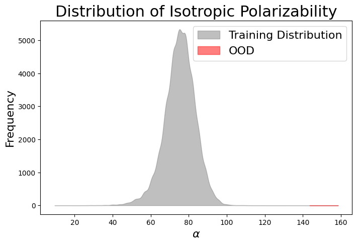
The model was initially trained conditionally on isotropic polarizability \(\alpha\) values \(x, h \sim p(x, h | c)\) drawn from the training distribution. During inference, generation was conditioned on out-of-distribution (OOD) property values (represented by the red extension of the distribution). Among the 100 molecules generated, only 38% were stable enough to run quantum mechanics (QM) calculations. The remaining molecules had issues such as incorrect charge or valency, rendering them completely invalid for QM simulations. Notably, the model appears to have generated some molecules with OOD isotropic polarizability values, as the histogram of the generated molecules \(\alpha\) extends beyond the OOD threshold!
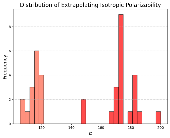
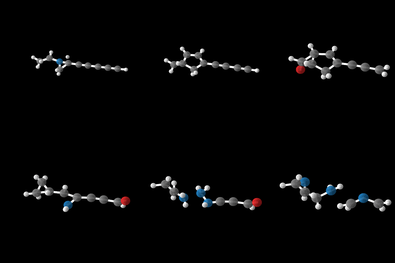
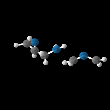
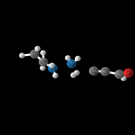
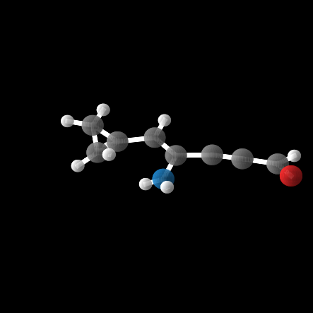
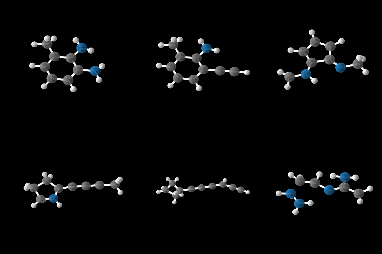
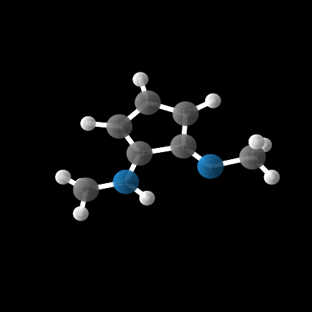
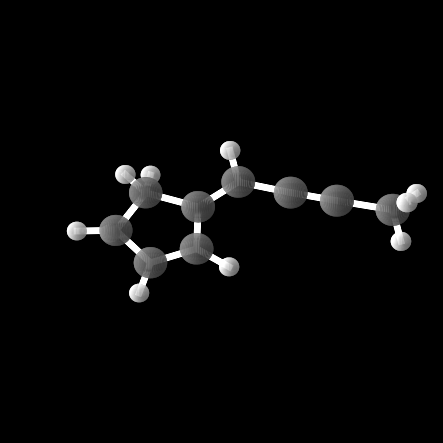
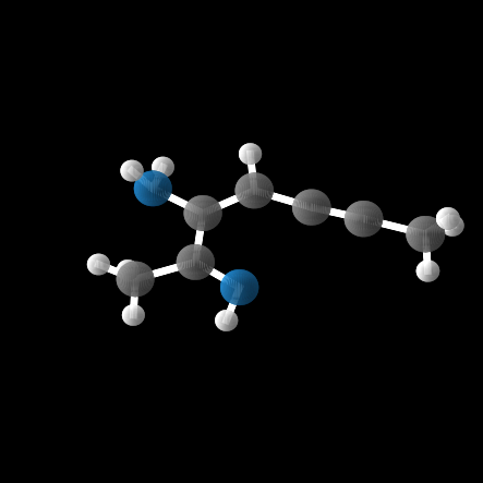
However, out of the 100 molecules generated, only 1% were valid molecules. Unfortunately, this single valid molecule had an isotropic polarizability of \(\alpha = 105.6\), placing it well within the distribution rather than in the OOD range. The remaining molecules exhibited incorrect bond lengths that would break the molecule in reality, as illustrated in the gif and figures below.
What about the top In-Distribution values?
It’s interesting to examine the model’s ability to generate molecules with extreme in-distribution (ID) values, as these samples are rare in the dataset. This highlights the model’s ability to generalize to cases that, although infrequent, were still seen during training.
In this case, 55% of the 100 molecules were stable enough for QM calculations, and 13% actually valid.

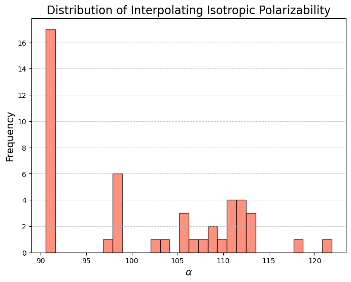
While the model was able to produce more valid molecules in the desired extreme \(\alpha\) range, the highest value was \(\alpha = 112.6\), far from the distribution edge.
Conclusion
When conditioning on values from the main distribution, the model’s validity reaches 90%, as reported in the paper. These results are not entirely surprising, as out-of-distribution (OOD) generalization is notoriously challenging for machine learning models. However, overcoming these challenges and improving OOD generalization for materials data remains a key area of research, as it holds the potential to drive significant advancements in materials design and the discovery of new, high-performance materials.
